Energy game manual
| Author: | Trevor Davis |
|---|---|
| Author: | Mark Thurber |
| Author: | Frank Wolak |
Thanks to Severin Borenstein and Jim Bushnell for developing the original "Electricity Strategy Game" that inspired and served as the original building block for this game. Thanks for the many participants in the 2013 and 2014 Stanford GSB class Energy Markets and Policy, participants to the 2013 Conference on Regional Carbon Policies, and participants in the 2014 course Best Practices in Electricity Market Design and Regulation who used earlier versions of the game and gave valuable feedback. Please don't hesitate to send feedback on this documentation to Trevor or on the Public issue tracker.
Contents
- Overview of games
- Energy game concepts
- Wholesale electricity markets
- Auction type: Pay-as-bid
- Auction type: Uniform price
- Cost-based bids
- Congestion in our game
- Hedging spot price risk
- Incentives with forward contracts
- Implementation of CPP-R in the game
- Demand conditions for the "days" in our game
- Base Genco portfolios
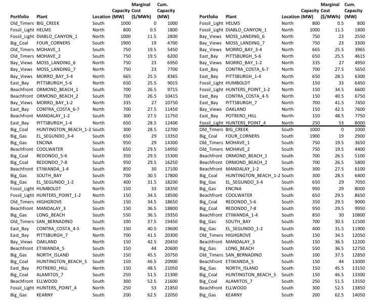
- Units ordered by marginal cost (overall and by region)
Overview of games
Base game scenario
This game is a basic game where each generation company places bids for the full capacity of each unit in their portfolio of power plants in a Uniform-price auction. The game is separated into a North and South market but initially there is no transmission constraint. The game contains four periods approximating the shape of demand over a day. The other games deviate from this base game in order to illustrate different properties of electricity markets.
"Pay as bid" scenario
In this game generators bid under a Pay-As-Bid auction. It illustrates the impact of auction mechanisms on market impacts.
"Congestion" scenario
This unit illuminates the effects of network congestion. This games adds a 750 MWh transmission constraint between the North and South regions to the base game.
"Forward markets" scenarios
This unit illuminates the effects of forward contracts on generator behavior. In addition to the conditions of the base game, this game gives pre-assigned non-sellable forward contracts to the generators at the beginning of the game. Unlike the base game, this game repeats the high demand conditions. The "low" variant gives the teams forward contracts that cover a lower fraction of their base capacity, the "medium" variant gives the teams forward contracts that cover a higher fraction of their base capacity similar to what they'd sell under a competitive market, and the "high" variant has the teams contracted for more than their capacity.
"Carbon tax" scenario
This unit illuminates the effects of a carbon tax on generator behavior. This game adds a carbon tax of $163 per ton. If generators bid marginal cost and demand is as expected the amount emitted should be equivalent to that in the carbon cap scenario.
"Carbon cap" scenario
This unit illuminates the effects of a carbon cap on generator behavior. This game adds a carbon cap and tradeable carbon allowances to the base game. If generators bid marginal cost and demand is as expected the amount emitted should be equivalent to that in the carbon tax scenario.
Energy game concepts
Wholesale electricity markets
- Generating companies bid in the capacity of their units
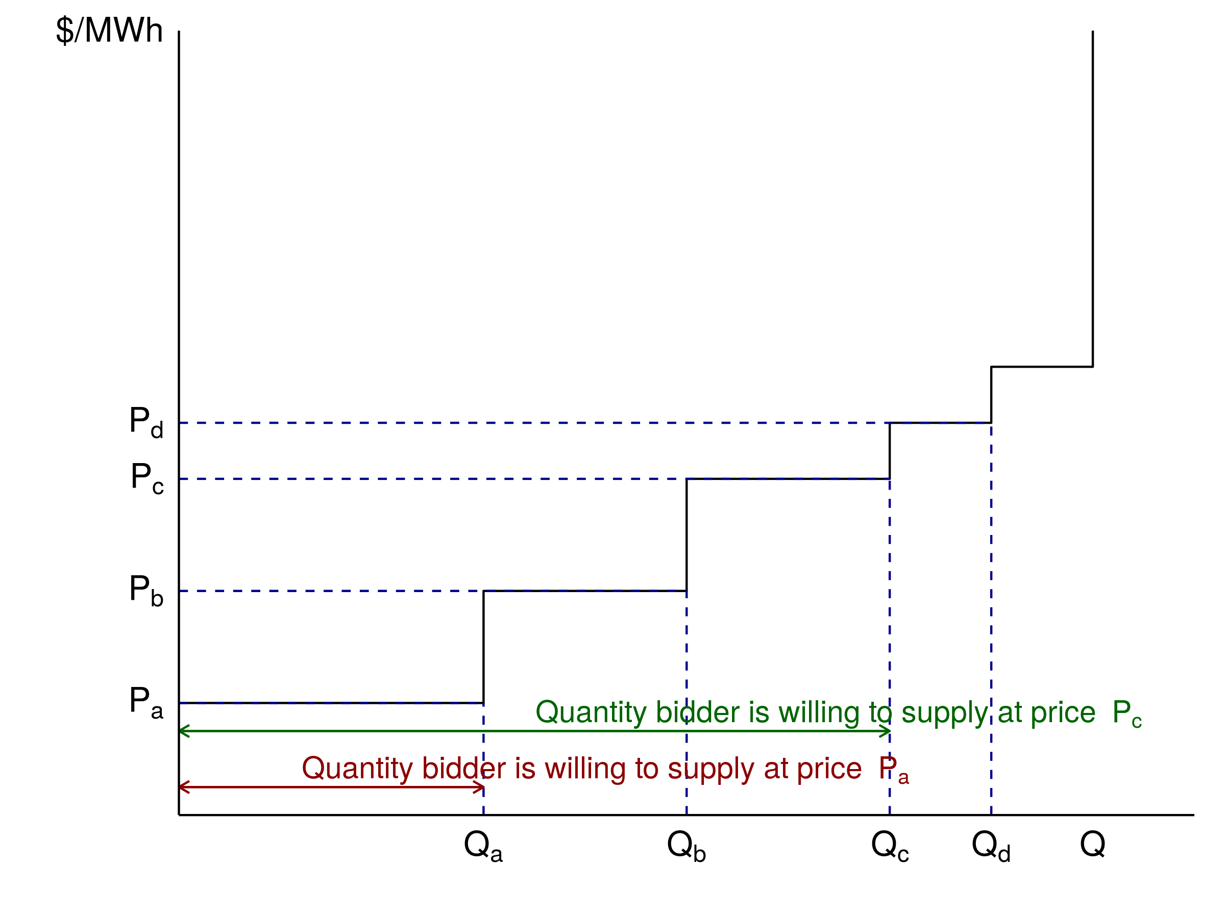
- System operator generates aggregate supply curve and crosses with demand to determine which plants run
- Various possible markets: e.g. day-ahead, day-of, hour-ahead (multi-settlement market has more than one type)


Congestion in our game
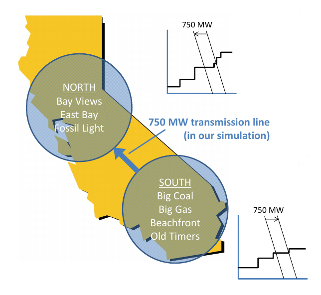
- Compute market equilibrium assuming no transmission constrain
- Compute how much power from one region would flow to the other
- If figure is greater than transmission line capacity, constraint binds
- Compute market equilibrium again, treating North and South as separate regions
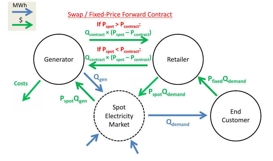
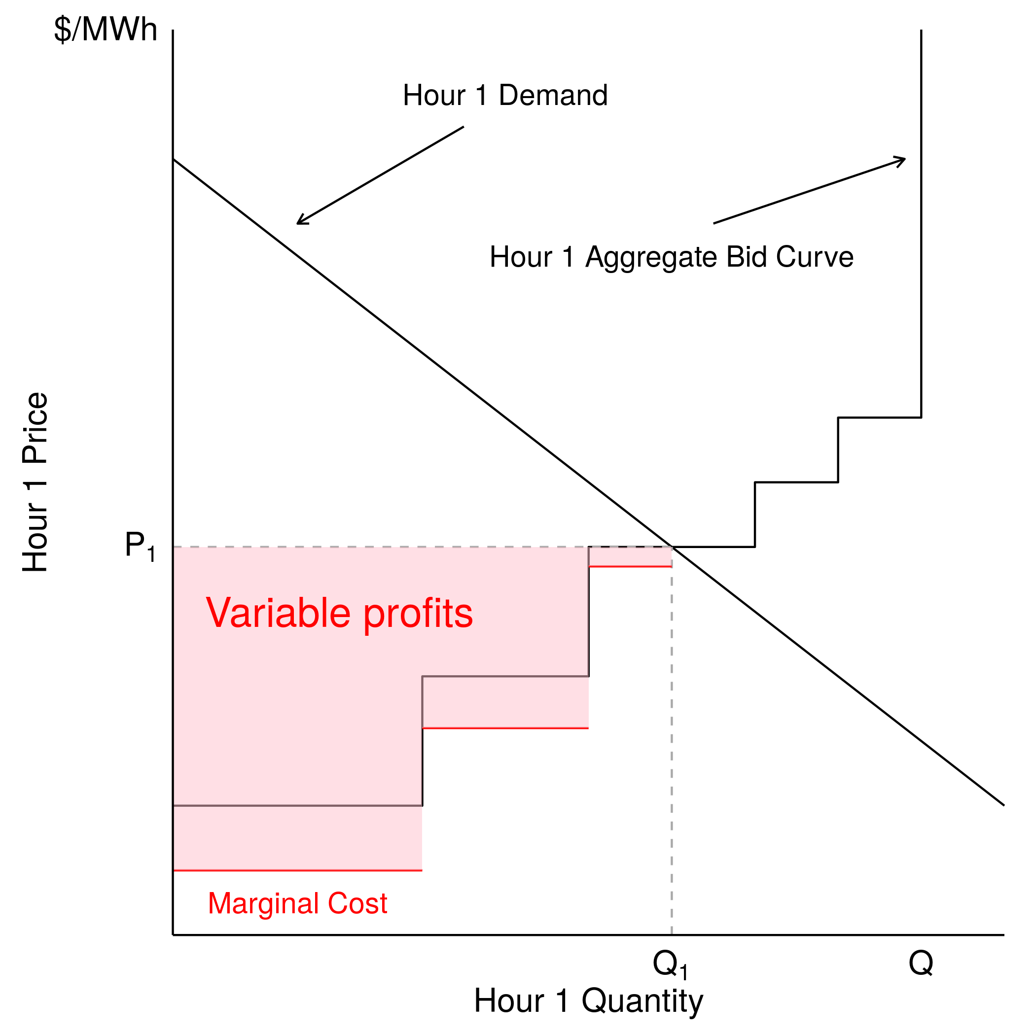
Incentives with forward contracts
Where
- (Qspot − Qcontract)*Pspot
- Revenue from selling electricity generated in excess of contracted quantity (or cost of purchasing electricity in the spot market to make up any shortfall relative to contracted quantity)
- Qcontract*Pcontract
- Revenue from forward contract
- Cost(Qspot)
- Cost of generating Q. This includes variable costs of operating units and fixed O&M of all units.
Implementation of CPP-R in the game
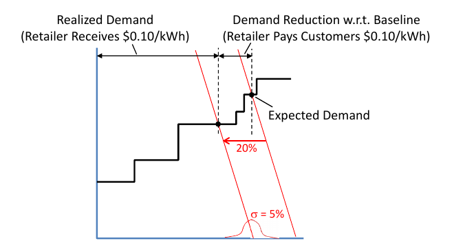
- Retailer declares CPP Rebate for next period
- Demand curve in next period is shifted in by average of 20% (std. dev. of 5%) - represents end customer response
- Retailer pays rebate to customers (say, $0.10/kWh)or reduction in demand relative to "expected"
- Retailer receives normal retail payment (say, $0.10/kWh) for realized demand
CPP-R helps retailers by substantially reducing procurement price (Pspot) if on a steep portion of the supply curve and also reduces demand in periods when Pspot > Pretail
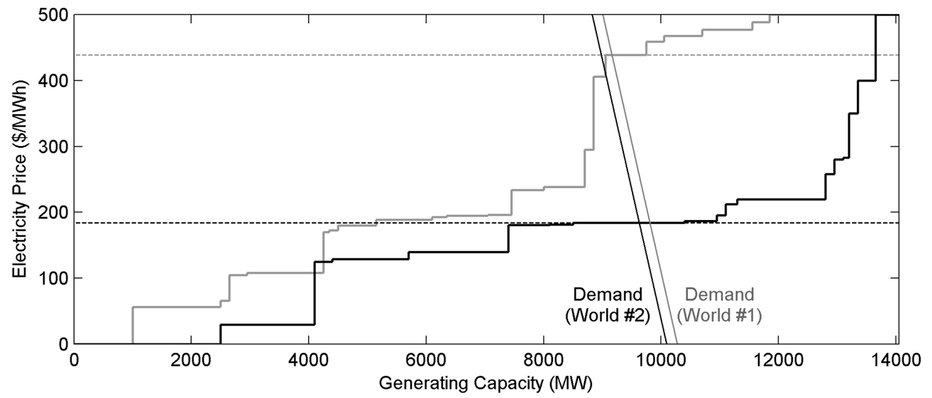
Demand conditions for the "days" in our game
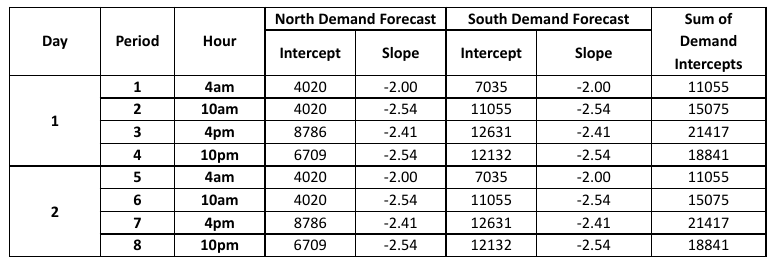
- Each period represents one "hour" of the day: 4am, 10am, 4pm, or 10pm
- Demand is relatively (but not completely) inelastic
- The realized demand intercept in both North and South regions is a random variable with mean equal to the forecast demand intercept and standard deviation equal to 3% of the forecast demand intercept
Base Genco portfolios
- portfolio:
- Name of the generating company that owns the plant.
- plant:
- Name of the power plant.
- location:
- Which region the plant is located in>
- mw:
- How much capacity (in MWh) does the power plant have.
- fuelcost:
- How much does it cost to buy the fuel needed to generate a MWh.
- varom:
- How much other variable "Operations and Maintenance (O&M)" costs are incurred per MWh produced.
- fixom:
- How much fixed O&M costs are incurred per period regardless of whether the plant ran or not.
- carbon:
- How many tons of CO2 are emmitted per MWh generated.
| portfolio | plant | location | mw | fuelcost | varom | fixom | carbon | type |
|---|---|---|---|---|---|---|---|---|
| Big_Coal | FOUR_CORNERS | South | 1900 | 17.5 | 1.5 | 2000 | 0.55 | coal |
| Big_Coal | ALAMITOS_7 | South | 250 | 50 | 1.5 | 0 | 0.59 | gas |
| Big_Coal | HUNTINGTON_BEACH_1-2 | South | 300 | 27 | 1.5 | 500 | 0.32 | gas |
| Big_Coal | HUNTINGTON_BEACH_5 | South | 150 | 45 | 1.5 | 500 | 0.53 | gas |
| Big_Coal | REDONDO_5-6 | South | 350 | 28 | 1.5 | 750 | 0.33 | gas |
| Big_Coal | REDONDO_7-8 | South | 950 | 28 | 1.5 | 1250 | 0.33 | gas |
| Big_Gas | EL_SEGUNDO_1-2 | South | 400 | 30 | 1.5 | 250 | 0.35 | gas |
| Big_Gas | EL_SEGUNDO_3-4 | South | 650 | 27.5 | 1.5 | 250 | 0.32 | gas |
| Big_Gas | LONG_BEACH | South | 550 | 36 | 0.5 | 500 | 0.42 | gas |
| Big_Gas | NORTH_ISLAND | South | 150 | 45 | 0.5 | 0 | 0.53 | gas |
| Big_Gas | ENCINA | South | 950 | 28.5 | 0.5 | 500 | 0.34 | gas |
| Big_Gas | KEARNY | South | 200 | 62 | 0.5 | 0 | 0.73 | gas |
| Big_Gas | SOUTH_BAY | South | 700 | 30 | 0.5 | 500 | 0.35 | gas |
| Bay_Views | MORRO_BAY_1-2 | North | 335 | 26.5 | 0.5 | 500 | 0.31 | gas |
| Bay_Views | MORRO_BAY_3-4 | North | 665 | 25 | 0.5 | 1000 | 0.29 | gas |
| Bay_Views | MOSS_LANDING_6 | North | 750 | 21.5 | 1.5 | 2000 | 0.25 | gas |
| Bay_Views | MOSS_LANDING_7 | North | 750 | 21.5 | 1.5 | 2000 | 0.25 | gas |
| Bay_Views | OAKLAND | North | 150 | 42 | 0.5 | 0 | 0.5 | gas |
| Beachfront | COOLWATER | South | 650 | 29 | 0.5 | 500 | 0.34 | gas |
| Beachfront | ETIWANDA_1-4 | South | 850 | 28.5 | 1.5 | 2000 | 0.34 | gas |
| Beachfront | ETIWANDA_5 | South | 150 | 42.5 | 1.5 | 250 | 0.5 | gas |
| Beachfront | ELLWOOD | South | 300 | 52 | 0.5 | 0 | 0.61 | gas |
| Beachfront | MANDALAY_1-2 | South | 300 | 26 | 1.5 | 250 | 0.31 | gas |
| Beachfront | MANDALAY_3 | South | 150 | 35 | 1.5 | 250 | 0.41 | gas |
| Beachfront | ORMOND_BEACH_1 | South | 700 | 26 | 0.5 | 1750 | 0.31 | gas |
| Beachfront | ORMOND_BEACH_2 | South | 700 | 26 | 0.5 | 1750 | 0.31 | gas |
| East_Bay | PITTSBURGH_1-4 | North | 650 | 28 | 0.5 | 625 | 0.33 | gas |
| East_Bay | PITTSBURGH_5-6 | North | 650 | 25 | 0.5 | 625 | 0.29 | gas |
| East_Bay | PITTSBURGH_7 | North | 700 | 41 | 0.5 | 1000 | 0.48 | gas |
| East_Bay | CONTRA_COSTA_4-5 | North | 150 | 40 | 0.5 | 250 | 0.47 | gas |
| East_Bay | CONTRA_COSTA_6-7 | North | 700 | 27 | 0.5 | 1500 | 0.32 | gas |
| East_Bay | POTRERO_HILL | North | 150 | 48 | 0.5 | 0 | 0.57 | gas |
| Old_Timers | BIG_CREEK | South | 1000 | 0 | 0 | 3750 | 0 | hydro |
| Old_Timers | MOHAVE_1 | South | 750 | 15 | 4.5 | 3750 | 0.47 | gas |
| Old_Timers | MOHAVE_2 | South | 750 | 15 | 4.5 | 3750 | 0.47 | gas |
| Old_Timers | HIGHGROVE | South | 150 | 34 | 0.5 | 0 | 0.4 | gas |
| Old_Timers | SAN_BERNADINO | South | 100 | 37 | 0.5 | 0 | 0.44 | gas |
| Fossil_Light | HUMBOLDT | North | 150 | 32.5 | 0.5 | 0 | 0.38 | gas |
| Fossil_Light | HELMS | North | 800 | 0 | 0.5 | 3750 | 0 | hydro |
| Fossil_Light | HUNTERS_POINT_1-2 | North | 150 | 33 | 1.5 | 250 | 0.39 | gas |
| Fossil_Light | HUNTERS_POINT_4 | North | 250 | 51.5 | 1.5 | 250 | 0.61 | gas |
| Fossil_Light | DIABLO_CANYON_1 | North | 1000 | 7.5 | 4 | 5000 | 0 | nuclear |